LLM From Scratch
Hi, in this blog, I will try to give an overview about LLMs stacks that can help you to land on any project requiring LLMs. I will go from core component of each LLM architecture, passing by how inference is done in LLMs. Then I will talk about finetuning LLMs on your own dataset or for your own tasks.
This post will be updated on a regular basis until it covers all possible aspect of LLMs
LLM architecture
Most of modern Large language models (LLMs) are based on decoder-only architecture. As illustrated in the figure below, every architecture use the same logic and workflow. They start with a tokenization step followed by an embedding layer, to produce a representation for each word in the input text. Then, they use a variant of Multi-Head Attention block (such as Masked Grouped Query attention in figure example, Multi-Head Latent Attention in models like DeepSeek V3/R1), Feed Forward block (containing Linear layers with activation function such as SiLU) and a Normalization Layer (e.g Layer Normalization, RMS Norm) to produce a general representation of the input text. This representation is finally passed through a linear layer to output a probability distribution over all the tokens in the vocabulary set of the LLM. This probability is used then to generate the next token. The generated token is added to the initial input text and the resulting in text is feeded to the LLM to generate the second next token until we have the full answer. This process makes LLMs autoregressive models which means to generate a token we need to process all the previous tokens.
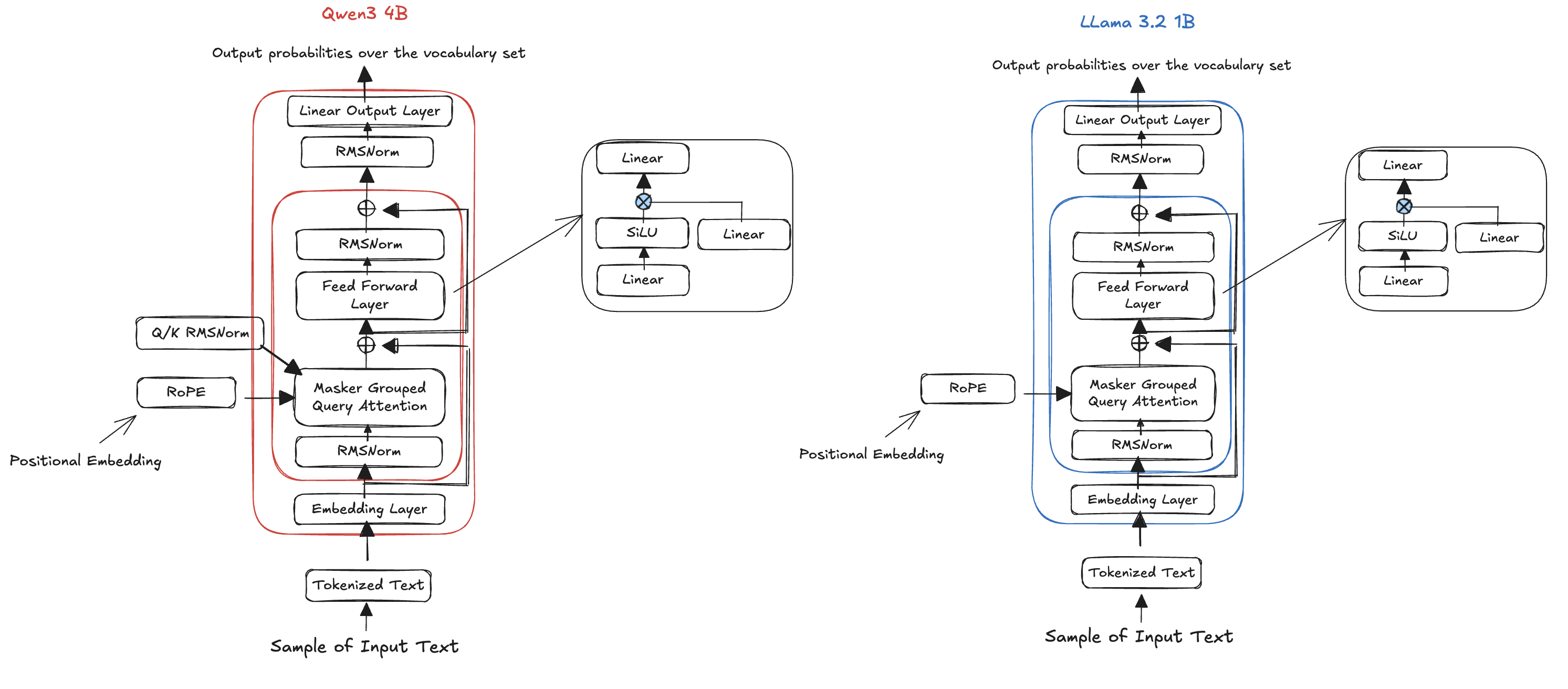
Figure: Scaled Dot-Product Attention
To have an idea about each component of an LLM, we will explain the original transformers architecture, which is an encoder-decoder architecture. As all models are based on that architecture and only slight changes made to it.
Transformers
Released by google in their paper “Attention is all you need” in 2017, transformers are backbone of modern LLMs architectures. They overcome Recurrent Neural Networks limitations. Prior to transformers, RNNs were the standards for sequential data such as text (e.g $s=(w_1, w_2, …, w_n)$ ). An RNN generates a hidden state $h_t$ for each element $w_t$ in the sequence by utilizing the element’s representation and the preceeding hidden state $h_{t-1}$. While this allows the model to capture context, it introduces a critical dependency: the computation for step $t$ must wait for step $t-1$. This sequential dependency causes significat issues:
- Inefficiency: Training cannot be parallelized across GPUs
- Instability: RNNs suffer from vanishing/exploding gradients.
- Information Loss: The context vector degrades over long sequences, failing to capture long-range dependencies.
Transformers solve these limitation by using a Multi-head attention mechanism to process input tokens in parallel, preserving relationships regardless of distance as illustrated in the figure below.

Let’s dig into the architecture of a transformer.
Input Embedding and positional Encodding.
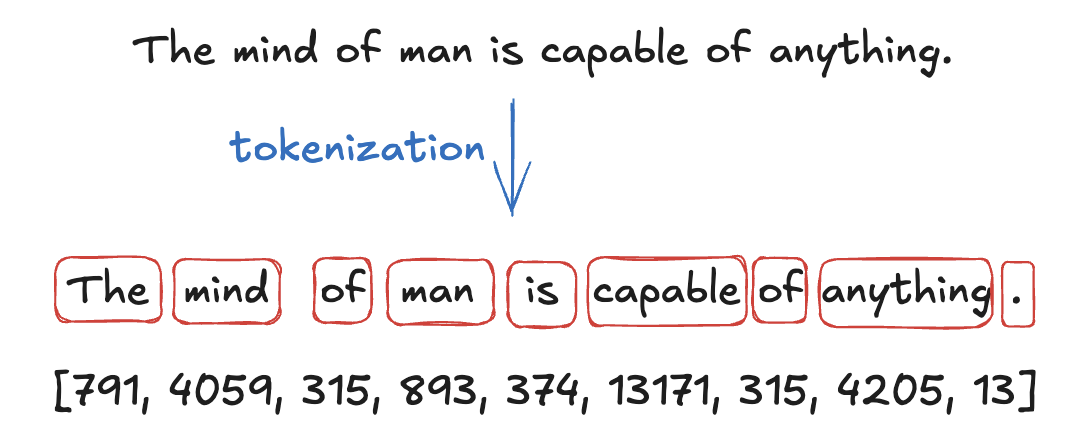
- From text to Tokens: The input to an LLM is a sequence of tokens ids, denoted as $s=(t_1, t_2, …, t_L)$ ($L$ represents the length of the sequence). These tokens ids are generated by a tokenizer (a process we will cover later), which takes the sentence and splits it into words or sub-words called tokens and finally each token is mapped to its own id. Each LLM have its own tokenizer, for example tokenizer of GPT is different from LLama and so on. The figure below ilustrate this process on the sentence “The mind of man is capable of anything.” (taken from heart of darkness by Joseph Conrad)
- The embedding Layer: Once tokenized, the sequence is passed through an embedding layer (it is learnable). This maps discrete tokens’ ids to dense vectors. If we assume the embedding dimension is $d_{model}$ (e.g $d_{model}=512$), this step outputs a tensor of shape $(L, d_{model})$. So, each token id $t_{i}$ is now represented by a dense vector of dimension $d_{model}=512$
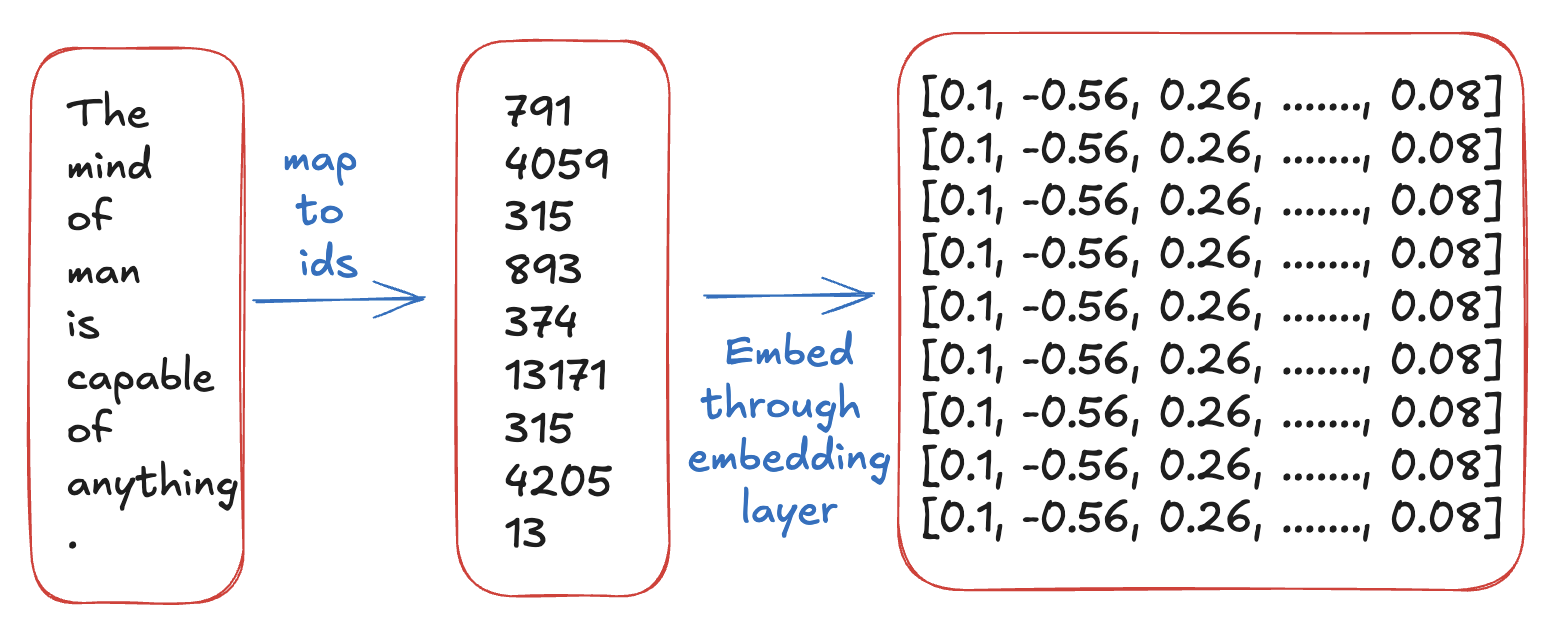
We can use nn module of pytorch to code the embedding layer as follows.
embedding_layer = nn.Embedding(vocab_size, d_model)
x_embedding = embedding(x)
- Positional Encodings: Here lies a critical challenge. Unlike RNNs, transformers process all tokens in parallel. This means the model has no inherent sense of order (it cannot distinguish between “the dog bit the man” and “The man bit the dog”). To solve this, we add Positional Embedding vector (not learnable) to each token’s embedding vector. This adds information about the token’s absolute or relative position in the sentence and help the model to understand the word function (whether it acts as noun, verb, subject etc). Without this, the Multi-Head Attention would view the sentence as a chaotic “bag of words” rather than a structured sequence.
#  Create a mtrix of shape (seq_len, d_model)
  pe = torch.zeros(seq_len, d_model)
  # Create a vector of shape (seq_len)
  position = torch.arange(0, seq_len, dtype=torch.float).unsqueeze(1) # (seq_len, 1)
  div_term = torch.exp(torch.arange(0, d_model, 2).float()*(-math.log(10000.0) / d_model))

  ## Apply sin
  pe[:, 0::2] = torch.sin(position*div_term)
  pe[:, 1::2] = torch.cos(position*div_term)

  pe.unsqueeze_(0) # (1, seq_len, d_model)
Multi-Headed Attention
As illustrated in the transformer architecture above, the input embedding and positional encoding block produce an input tensor $X$ of size $(L, d_{model})$ which contains a dense vectors representing tokens in the text sequence. This input tensor is feeded then to Multi-Head Attention block to capture token’s interaction with other words. Multi-head Attention block is based on Scaled Dot-Product Attention, which we will explain first.
Scaled Dot-Product Attention The scaled Dot-Product attention takes as input three matrices of size $(L, d_{model})$: Queries $Q$, Keys $K$ and Values $V$. Those three matrices are just the input tensor (often via linear projection) where:
\[Q = X \qquad K = X \qquad V = X\]The mechanism then compute a new representation for each token, enriching it with contextual information from other tokens using The following formula and the figure below illustrate the mechanism:
\[Attention(Q, K, V) = softmax(\frac{QK^{T}}{\sqrt(d_k)})V\]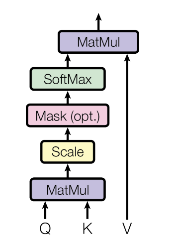
Figure: Scaled Dot-Product Attention
- Similarity: $QK^{T}$ calculates the similarity between every Query and every Key
- Scaling: We divide by $\sqrt d_k$ to prevent gradients from vanishing in the softmax.
- Weighting: The softmax turns the scaled similarities into attention scores (or probabilities) representing how relevant every other token is to the current token. Multiplying these scores by the V matrix produces a weighted sum of the value embeddings.
Properties:
- Permutation invariant: Attention mechanism is mainly matrix computation. It does not inherently respect the order of the sequence. Changing row order of input will output the same results. This is why positional embedding is required.
- Masking: The score matrix yielded by the Softmax operation has a size of $L \times L$. If we want to prevent interactions between some tokens (like hiding future tokens during training), we apply a mask - setting those scores to $-\infty$, before applying the softmax function, so their probabilities become zeros.
def attention(query, key, value, mask):
  d_k = query.shape[-1]
  attention_scores = query@key.transpose(-2, -1) / math.sqrt(d_k)
  if mask is not None:
      attention_scores.masked_fill_(mask==0, -1e9)
  attention_scores = attention_scores.softmax(dim=-1)
  output = attention_scores@value
  return output
Multi-head Attention Multi-HEad attention refines the mechanism and improves the model’s performance by allowing it to jointly attend to information from different representation subspaces at different positions.
Instead of performing single attention $d_{model}$-dimensional matrices, it is benificial to linearly project the Q, K, and V matrices $h$ times with different, learned linear projections to $d_k$, $d_k$, $d_v$, respectively.
A scaled dot-product attention is performed on each of the $h$ projected versions of Q, K, and V, yielding $d_v$-dimensional output values. These are concatenated and once again project to result in the final values. The following formula and figure illustrate the process:
\[MultiHead(Q, K, V) = Concat(head_1, ..., head_h)W^{O}\] \[head_i = Attention(QW_{i}^{Q}, KW_{i}^{K}, VW_{i}^{V})\]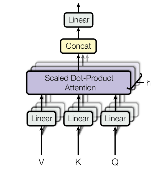
Figure: The Multi-Head Attention Mechanism
W_q = nn.Linear(d_model, d_model)
W_k = nn.Linear(d_model, d_model)
W_v = nn.Linear(d_model, d_model)
W_o = nn.Linear(d_model, d_model)

query = W_q(q)
key = W_k(k)
value = W_v(v)

B, seq_len = query.shape[0], query.shape[1]

query = query.view(B, seq_len, h, d_k).transpose(1, 2)
key = key.view(B, seq_len, h, d_k).transpose(1, 2)
value = value.view(B, seq_len, h, d_k).transpose(1, 2)

x = attention(query, key, value, mask)
x = x.transpose(1, 2).contiguous().view(B, seq_len, d_k*d_h)
x = W_o(x)
Add & Norm Layer and Residual connection
The output of the multi-head attention block is a tensor $M$ of size $L \times d_{model}$ which is passed to Add & Norm layer. In this layer the input tensor $X$ is added to $M$ via a residual connection. This addition or residual connection prevents from vanishing gradient. Then the output of this addition is normalized.
Either in the original transformer paper the Norm layer is placed after the attention block or the feed forward layer, known as Post-Normalization, many LLMs architecture use the normalization layer before, known as Pre-Normalization. In 2020, Xiong et al, they showed thatPre-Normalization is more benificial by resulting in more well behaved gradients at initialization and works well without careful learning rate warm-up which is critical for Post-Normalization.
In some LLMs such as OLMo 2, they use Post-Normalization with RMSNorm instead of Layer Norm or Batch Norm as it results in smoother gradients and then more stability in the training.
Feed Forward Layer
Decoder
The decoder is similar to the encoder. It takes the outputs as input and pass them through embedding and position encoding block. The tokens’ tensor is passed as Queries, Keys and Values, through a Masked Multi-head Attention. The output of the Masked Multi-head Attention is passed as Queries to another Multi-Head Attention along with the encoder output which is considered as Keys and Values.
The goal of using Masked Multi-Head Attention is to make the model causal (i.e the output at a certain position can only depend on the words on the previous position). The model must not be able to have information about the future. This is achieved by using the masking property of Scaled Dot-Product Attention. The scores that correspond to the current token and its interaction with future tokens are set to $-\infty$ which will yield to 0 when applying softmax.
Linear and softmax
proj = nn.Linear(d_model, vocab_size)
out = torch.log_softmax(proj(x), dim=-1)
Training
Training an LLM is done through two steps: Pre-training step which consists of training the LLM on a large scale data (billions to trillions of tokens). The result of this step is a base model and it aims only to encode the world knowledge into the models. This means it can generate token in a way to have meaningful generation but not necessarly correct. For example if we ask the base model “when was the first LLM trained” and it answers “1439”, it gives a good output but it does not matter if it is true. This step is very expansive as it requires powerful resources that scale up with model’s number of parameters and the data.
The Second step is Post-training step which consists of training the base-model on high quality data to align its behavior imporve its capabilities and make it more helpful. For post-training, we can use mainly Supervised fine-tuning (SFT) or reinforcement learning (RL).
Pre-training and SFT consists of optimizing the same loss function and reiforcement learning use different loss function. But the training logic is mainly the same. We will details how we train an LLM in general and then we will give some examples of loss function for RL. \
| The goal of a language model is to predict the probability of the sequence of tokens. Let ${x_1, x_2, …, x_n}$ be our sequence. Its probability is $Pr(x_1, x_2, …, x_n) = \prod_{i=1}{n} Pr(x_i | x_0, x_1, …, x_{i-1})$. |
| When applying the log the sequence probability becomes : $\log Pr(x_1, x_2, …, x_n) = \sum_{i=1}{n} \log Pr(x_i | x_0, x_1, …, x_{i-1}$. |
So, predicting the next token, we mainly want a token having the highest probability as follows: $\hat{x_i} = argmax{x_i \in V} Pr((x_i|x_0, x_1, …, x_{i-1})$.
In SFT, the data is composed from input context $x = {x_1, x_2, …, x_n}$ and the desired output $y = {y_1, y_2, …, y_T}$. The SFT is a multiclass-classification problem, the loss function used is negative log-likelihood of producing the correct sequence $y$ given the input $x$. This is often implemented as cross-entropy between the predicted class by the model and the true class in the dataset.
At seqeunce step $t$, let $y^{}_{t}$ the ground truth token and let $\log p_{\theta}(y^{}{t}|x_1, …, x_n, y_1, …, y{t-1})$ denote the log-probability of producting the token $y^{*}_t$ by the model.
Then the model optimizes the following Loss function:
| $L_{SFT}(\theta) = -E_{(x,y)~D} \sum_{t=1}^{T} \log p_{\theta}(y_{t} | x_1, …, x_n, y_1, …, y_{t-1})$ |
in Practice we use the following formulation: $L_{SFT}(\theta) = -\frac{1}{T} \sum_{t=1}^{T} \log p_{\theta}(y^{*}{t}|x_1, …, x_n, y_1, …, y{t-1})$
Intuition: The following loss is trying to maximize always the probability of the ground truth token $y^{*}_{t}$ and push it to be 1. The log is applied on the probabilities which have values between $0$ and $1$, so the -log gives values between $+\infty$ and $0$. So minimizing this loss means pushing the -log to be 0 and then the probabilities to be 1.
Inference
| At inference, we have a context $x = {x_1, x_2, …, x_n}$ and we want to generate a sequence $\hat y = {y_1, y_2, …, y_T}$ such that $Pr(\hat y | x) = \prod_{t=1}{T} Pr(y_t | x_0,…, x_{n}, y_0, …, y_{t-1})$ is maximal. So the generation process is as follows: at eacht time step $t$ we generate a token $y_t$ using its conditional probability $Pr(y_t | x_0,…, x_{n}, y_0, …, y_{t-1})$. Add the generated token to the context which is use after to generate the next token $y_{t+1}$. But how do we use the conditional probabilities to generate the next token? |
Greedy Search Strategy: This strategy consists of selecting the token with the highest conditional probability at each time step $t$: $\hat y_{t} = argmax_{y_t \in V}{Pr(y_{t} | x_1, …, x_n, y_1, …, y_{t-1})}$
Selecting always at each time step $t$ the token with the highest probability does not entail that the the entire output sequence has the maximum joint probability. Maybe selecting the second probable token at time step $t$ could lead to have token with higher probability at timestep $t+1$ than a token yielded by selecting the first probable token at timestep $t$.
So, while this method is efficient as it sees at each timestep $t$ one token (the most probable token) comparing to other methods that take into account many tokens and keep track of them to generate the sequence (will be explained later). It can miss better tokens as explained above and lead to short-sighted output.
| Beam Search: At each timestep $t$ we select $n$ first probable tokens ($n$ is the number of beam). This process is repeated until we reach the predifined maximum length $T$ or end-of-sequence token appears. Then, we will choose the sequence $y$ that have maximum joint probability $P(y | x)$ |
Top-k sampling strategy: It leverage the probability distribution generated by the language model to select a token randomly from the k most likely options. This method add an element of randomness in the generation process.
You might hear that temperature controls the creativeness of the LLM. Higher temperature more creative model and lower temperature more deterministice model. Actually, the temperature add another sort of randomness in the generation process. It affects the shape of the probability distribution. The probability distribution is formulated as follows:
$softmax(x_i) = \frac_{e^{\frac_{x_i}{T}}{\sum_{j}e^{\frac_{x_j}{T}}}$
So, higher temperature encourages the probability distribution to be near to a uniform distribution. This is why higher temperature lead to hallucination. Lower temperature increases the probability of the most probable tokens and decreases the probability of unlikely tokens.
If we use top-k sampling strategy with lower temperature, we will likely sample the same sequence if we call the LLM many times.
Nucleus sampling strategy: known also as top-p sampling. At each timestep $t$, it consists of selecting top probable tokens in a descending way until their cumulitive probabilities exceeds a cutoff values $p$. Then, the next token is sampled from the selected tokens. Using this strategy, we have at each timestep $t$ a different number of tokens to select from. This encourages more diverse and creative output.
Quantization:
Large Language Models require powerful resources to generate a response in a reasonable time as they get bigger and have more parameters. Not only the number of parameters that influences the quantity of computational resources needed, but also the data type of the parameters affects and the efficiency of the model. Generally in deep learning, and in LLMs specifically, FP32, FP16 and BF16 are used as data types:
- FP32: Uses 32 bits to represent a number. One for the the sign, eight for the exponent, and the remaining for the significand. This data type provide a high degree of precision but it is computational high and memory footprint.
- FP16: Uses 16 bits to represent a number. One bit for the sign, five for the exponent and 10 for the significand. It is more memory efficient and less computational but it introduce numerical stability and potentially impact the model performance due to the reduced range and precision in representing the number.
- BF16: Uses also 16 bits to represent a number. One for the sign, seven for the exponent and 8 for the significand. It expands the representable range compared to FP16, thus decreasing underflow andoverflow risks. Despite a reduction in precision due to fewer significand bits, BF16 typically does not significantly impact the model performance.
As you can conclude, using 1B model with FP32 or FP16 will come with a tradoff between accuracy and memory footprint and latency. Depending on the use case, we can have the accuracy needed with data types that are computational lower than FP16, such as INT8 or INT4. The model parameters (weights) are generally in FP32 and converting them to a lower-precision data type such as INT8 or INT4 is called Quantization.
Generally, we have two types of Quantization:
- Post-Training Quantization (PTQ): It is straightforward technique where the weights of an already trained model are converted to a lower-precision data type.
- Quantization-aware training (QAT): incorporate the quantization process during training stage of finetuning. QAT is computational expensive and requires representative training data.
Let’s get an intuition by introducting some naive-quantization 8-bit techniques.
Absolute Maximum Quantization (absmax): It uses the following formula to convert an FP32/FP16 number to INT8 number:
\(X_{quant} = round(\frac{127}{\abs{X}}.X)\) \(X_{dequant} = round(\frac{max(\abs{X})}{127}.X_{quant})\)
This methods is symetric and it maps weights values to a range of $[-127, 127]$
This methods comes with a loss of precision due to rounding. When applying the dequantization formula to get the original weights, we will have a precision error.
Zero-Point Quantization: It applies the following formula to perform quantization.
\(scale = \frac{255}{max(X) - min(X)}\) \(zeropoint = -round(scale . min(X)) - 128\) \(X_{quant} = round(scale . X + zeropoint)\)
\[X_{dequant} = \frac{X_{quant} - zeropoint}{scale}\]This methods is asymetric and maps the weights value to a range of $[-128, 127]$
In practice, we apply vector-wise quantization which consider the variability of values in rows and columns of the same Tensor. Quantizing the entire Tensor in one pass will lead to a huge model degradation and quantizing individual values will yield to a big computation overhead.
The both methods discussed above are sensitive to outliers.